Today, I will be covering the DSP part of the SDR processor, using my laptop to generate IQ signals that we could then use in practice to transmit signals over the air! This will also be a series to creating our own fully function SDR transceiver!

This marks the beginning of a entire series where I’ll be designing and creating a fully funtional SDR transceiver! This entry will be mostly theory and the beginning of basic SDR concepts.

I became licensed for amateur radio a little more than a year ago! I bought a old brick of a ICOM IC-730 that still somehow functions great today.

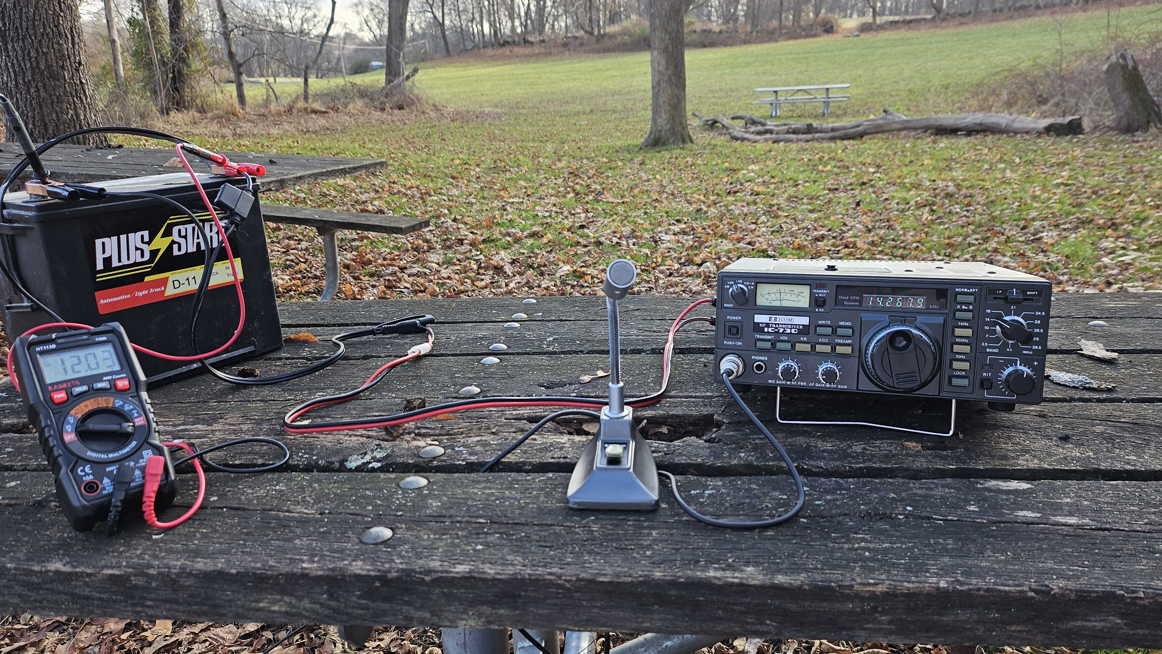
Here’s a photo of the radio setup at a park for a POTA (Parks on The Air) operation. It worked great and made ~15 contacts!

Anyway, That thing is from the 80s and lacks a lot of modern features radios have today. However before continuing, let’s get some abbreviations and definitions out of the way first! I don’t wanna confuse you guys.

Here a lot of things I’ll be saying:

• IQ - In-Phase and Quadrature
• SDR - Software Defined Radio
• PSK / BPSK - (Binary) Phase Shift Keying
• Constellation - A grid that graphs the I and Q components
• AM - Amplitude Modulation
• VFO - Variable Frequency Oscillator
• LO - Local Oscillator
• DSP - Digital Sound Processor
• RF - Radio Frequency
• FFT - Fast Fourier Transform

Now that’s out of the way, let’s get into the cool new radios! Older radios, pre 2000s, were mostly analog. They likely had a Digital VFO, which increased frequency stability. A VFO is the knob you’d turn to change the frequency radio, it acts as the Local Oscillator that the radio would use to modulate and demodulate signals. Other than that, modulation, demodulation, and everything in between was strictly analog with transistors, capacitors, inductors, resistors and some more. Here’s a block diagram of how this would look:

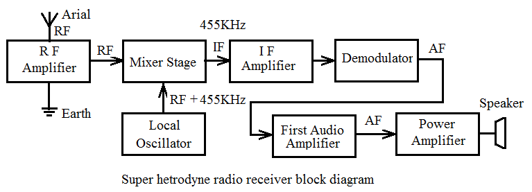
Figure 1.0 - Superheterodyne receiver block diagram

Many radios today still use this architecture, like alarm clocks, your car, just to name a few. This is a superheterodyne receiver. These receivers use an Intermediate Frequency to lower the frequency of the signals to something that is more convenient to work with. Common with AM radios, they lower the 500KHz-1.6MHz signals down to 455KHz, which is a lot easier for common components to handle.

This was discovered in the early 1900s by Edwin Armstrong. If you want to receive a signal at 1000KHz, but your hardware can only efficiently work with 445KHz, then you can tune the LO to 1445KHz, and since summing two sine waves results in the sum and the difference, there is now the same signal being broadcast 1000KHz at 445KHz and 2445KHz. This is genius, and allows the receiver to only have to listen to one specific frequency, in this case 445KHz, while tampering with the LO’s frequency will change the signal that appears at 445Khz. The receiver now only needs to be capable of listening at 445Khz, yet able to listen to a plethora a new signal without actually needing the ability to amplify or demodulate at that new high frequency.

The superhet Wikipedia entry has a great history and explanation of this.

This is still widely used today, even with new SDR systems. However in transceivers this has been mostly phased out into Software Defined Radios (SDR). SDR takes a whole different approach, and instead modulates and demodulates signals using math from software on a computer, then output using a Digital to Analog converter. Here’s how that would look:

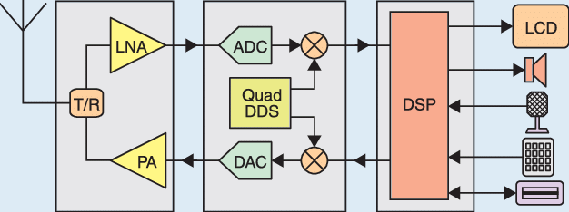
Figure 1.1 - Direct Sampling SDR block diagram

Now this is pretty simplified, as there are many different types of SDR, but this is the basic principle. The Quad DDS can be relabeled as a Local Oscillator to make more since. The DSP outputs a modulated baseband signal which is then mixed with the LO to get it up to RF frequencies.

That diagram would represent a Direct Sampling SDR, as it directly samples the signals at a specific frequency. Also common with SDR is a superhetero design, where the ADC samples the Intermediate Frequency instead. A Low Noise Amplifier is required as most ADCs cannot accurately detect the sub-microvolt changes in amplitude that an antenna would pick up.

Another common type is a Direct Conversion Receiver, which is the same as a superhet receiver, but instead has the LO identical or very close to the signal of choice, make the signal baseband.

SDRs are technically limited by how good the ADCs and DACs are, but are also limited by the quality of the software written for them.

Today, I will be covering the DSP part of the SDR processor, using my laptop to generate IQ signals that we could then use in practice to transmit signals over the air! This will also be a series to creating our own fully functional SDR transceiver!

Getting into the signals

So working with SDR’s requires a pretty good understanding of calculus principals and other goofy math stuff.. It’s actually not too complex though! First let’s talk about AM, and the math behind it!

What are IQ signals?

In simple terms, any modulated sinusoidal can be represented by or composed of two Amplitude Modulated sinusoidal that are 90 degrees out of phase.

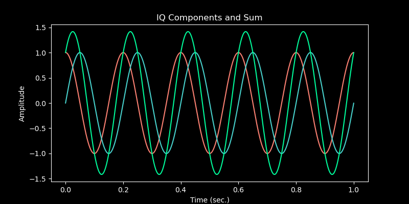
Figure 2.0 - IQ Components and Sum

In this diagram, the the red cosine is the I component, the blue sine is the Q component, and the green 45 degrees out of phase sinusoidal is the sum of the IQ components.

A big idea with this is that the modulated data can be treated separately from the carrier, which is a big deal in some modulations. This will also be used a lot in digital radio modes because the I and Q components can carry separate data. A constellation is the I and Q components graphed out on a coordinate grid.

This concept is used everywhere in Software Defined Radio, and will be mentioned frequently.

IQ files

IQ data is simply just an array or list of complex numbers. For example, [0.23 + j0.54, 1 + j0.32, 0.65 + j0.82, ...] Those numbers are just [I+jQ, I+jQ, I+jQ, I+jQ, ...]

Note: j just represents the complex factor of the number.

Binary File

A popular IQ file format is just a binary file in the format IQIQIQIQIQIQ, where each component is a float being stored one after another. It is recommended to use the.iq extension to denote this. The biggest issue with this method is that there is no metadata with the data, so you manually would have to put the sampling rate and frequency into the software.

To fix this, the community created a standard called SigMF. SigMF metadata is stored alongside the IQ file in a file named file-name.sigmf-meta. The IQ file should also be renamed to file-name.sigmf-data. The filename should be the same, but with different extensions. I wont go over this in depth, but here’s an example configuration:

{
 "global": {
 "core:datatype": "cf32_le",
 "core:sample_rate": 1000000,
 "core:hw": "PlutoSDR with 915 MHz whip antenna",
 "core:author": "Art Vandelay",
 "core:version": "1.0.0"
 },
 "captures": [
 {
 "core:sample_start": 0,
 "core:frequency": 915000000
 }
 ],
 "annotations": []
}

SigMF allows for annotation when visually analyzing the signal, giving a description, hardware your using, sample rate, the format of the IQ file, and much more! It a really great standard, and I recommend looking into it much more over at the SigMF website!

Wave Container

Another popular way to store IQ data is using a wave file. It uses two channels to store the IQ data as a 16 bit integer, the the left and right channel being the I and Q component respectively. The sampling rate of the wave container is how to software will handle the IQ signal. This method can be considered a little dangerous, since the file can be played through normal audio players, which may damage some audio systems.

We will be utilizing both of these methods later on!

What is modulation?

Well, sorry, I’ve been using that word a lot wth explaining my self. Modulation is the principle of taking some form of continuous wave carrier signal, such as a sine wave at a given frequency, and varying some variable of that carrier with a information bearing signal, such as audio data, binary data, etc.

Now what the hell does that mean? Well, let’s take a sine wave with a frequency of 1000hz. That’s our continuous wave carrier signal, and if we vary the amplitude of that sine wave by another one, say a 200hz sine wave, that’s a Amplitude Modulated signal!

Frequency modulation varies the frequency of a sine wave to convey information, and PSK varies the phase of a sine wave to convey information.

Let’s go make more sense of this in the Amplitude Modulation section!

Amplitude Modulation

AM is the first modulation mode ever used to transmit audio, dating all the way back to the 1900s. It is continued to be used today due to it being extremely simple in principle and easy to receive and transmit. Due to information being conveyed in amplitude, it is quite affected by noise.

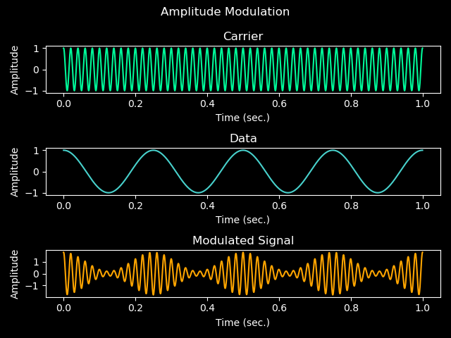
Figure 2.1 - Amplitude Modulation Components

Here’s a diagram of the individual components of a AM signal. As you can see, the modulated signal has a amplitude the corresponds to the data signal. This is the basic premise of AM.

We can also look at the FFT, which will show us that modulated signal in the frequency domain.

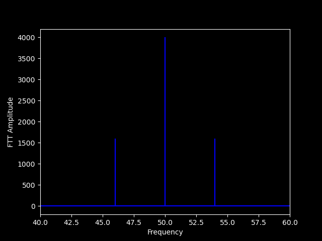
Figure 2.2 - Amplitude Modulation in the Frequency Domain

Here you can see the visual representation of a AM signal in the frequency domain. We can see the carrier frequency clearly at 50hz, along with both of the sidebands, being +/- 4hz away from the carrier, which is our data signal! There are sidebands because without them, out signal would just be a single carrier at 4hz. Adding two sine waves results in the sum and the different of the frequencies.

The biggest disadvantage of AM also shows by looking at this FFT graph. As you can see, most of the power is being put into the carrier, which conveys no information. This is about 2/3rd of the power being wasted, with the rest going into the actual signal. AM is only 33% efficient. People have created different modes, like DSB-SC, or Dual Sideband Suppressed Carrier which keeps the sidebands but removed the carrier completely. This increases efficiency to 50%! There is also SSB-SC, Single Sideband Suppressed Carrier which is technically 100% efficient! In practice though, it is harder to tune, requires accurate oscillators and is very much effected by noise. It is the most popular mode for voice in amateur radio. SSB is practically baseband but mixed to a different frequency.

The Math Behind Amplitude Modulation

Now that we know how an AM signal works, we can finally start creating one!
The carrier is the simplest to create, as it’s a pure sinusoidal. We can represent a carrier wave as:

\[c(t) = cos(\omega t)\]

\[c(t) = cos({2}\pi{ft})\]

Where \(\omega\) = angular frequency in rad/s, \(t\) is time, and \(f\) is frequency in hertz. \(\omega\) is equal to \({2}\pi{f}\)

With this, an AM signal can be represented as:

\[ m(t) = A(t) * cos({2}\pi{f_ct})\]

Where \(A(t)\) is the change in Amplitude over time, and \(f_c\) is the carrier frequency in hertz.

As an example, the example in Figure 2.1 can be represented as:

\[y(t) = [1 + mcos({2}\pi{4}t)] * cos({2}\pi{50}t)\]

Here, \(m\) is the modulation index. The modulation index is how modulated the signal is.

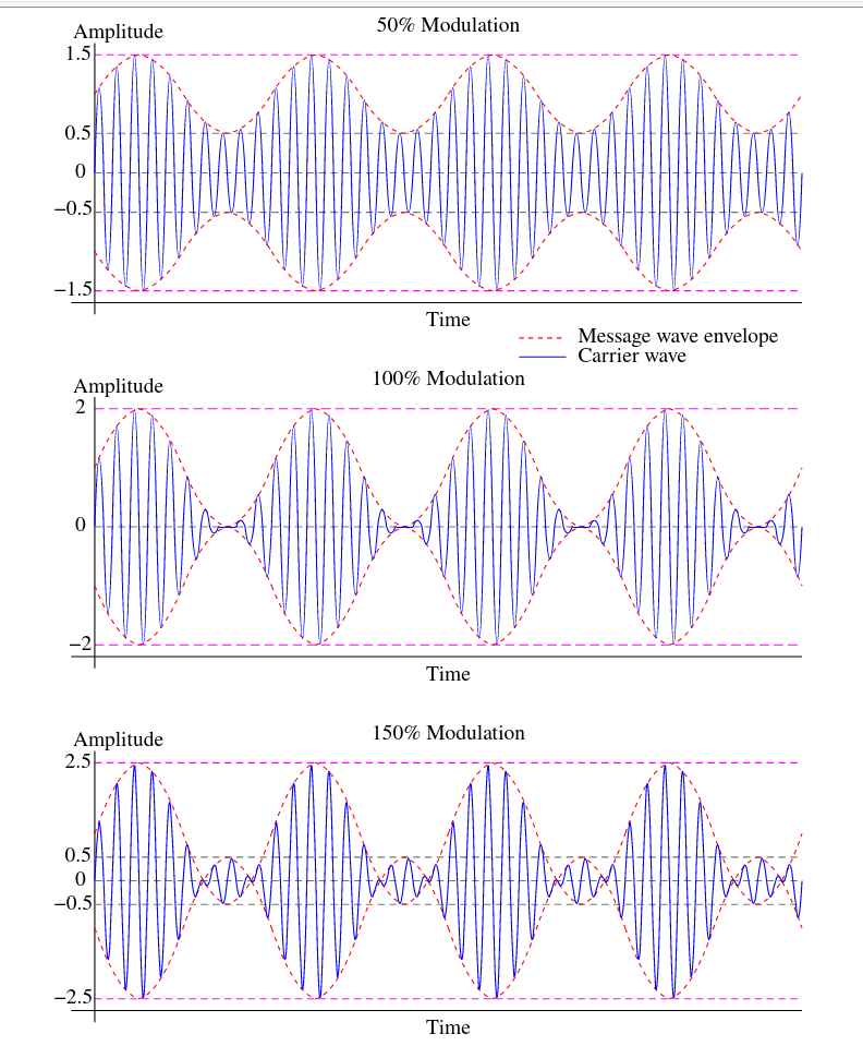
Figure 2.3 - Modulation Index

That’s it! AM is probably the simplest modulation you will ever encounter, other than CW (Morse Code).

Creating AM signals in Python

Using Python, we can easily create these IQ signals and export them to files that SDR software can recognise. Let’s get started! We’ll recreate Figure 2.1.

First we want to be sure to import numpy

import numpy as np

When working with SDR, there will always be a sampling rate. This is how often the waveforms will be samples, and this must be at least double the largest frequency you want to represent due to the Nyquist Theory.

We will use 8000, as that is common for early DSP microcontrollers and covers the maximum allowed amateur bandwidth of 3KHz.

In this I will also define the length to be 1 second, and user np.arange to create an array of time values for every sample in between 0 and 1 seconds at a 8000hz sampling rate.

sampling_rate = 8000
duration = 1
t = np.arange(0,duration,1/sampling_rate)

Now let’s create the carrier and data wave. We’ll just be copying those equations above.

carrier = np.cos(2 * np.pi * 50 * t)

data = np.cos(2 * np.pi * 4 * t)

Perfect! Now we have a carrier at 50hz and a 4hz tone. Let’s modulate it as is above”

modulation_index = 0.85 # 85%
modulated = (1 + (modulation_index * data)) * carrier

Now we have our Amplitude Modulated signal! We can graph it out with matplotlib and get a image very similar to Figure 2.2

import matplotlib.pyplot as plt

fig, (ax1, ax2, ax3) = plt.subplots(3,1)
fig.suptitle("Amplitude Modulation")
fig.set_tight_layout(True)

ax1.plot(t, carrier, color="mediumspringgreen")
ax1.set_title("Carrier")
ax1.set_xlabel("Time (sec.)")
ax1.set_ylabel("Amplitude")

ax2.plot(t, data, color="mediumturquoise")
ax2.set_title("Data")
ax2.set_xlabel("Time (sec.)")
ax2.set_ylabel("Amplitude")

ax3.plot(t, modulated, color="orange")
ax3.set_title("Modulated Signal")
ax3.set_xlabel("Time (sec.)")
ax3.set_ylabel("Amplitude")

fig.show()

Awesome! We have exactly what we want now. Let’s run it:

Figure 2.4 - Python Output 1

The final code:

import numpy as np
import matplotlib.pyplot as plt

sampling_rate = 8000
duration = 1
t = np.arange(0,duration,1/sampling_rate)

carrier = np.cos(2 * np.pi * 50 * t)

data = np.cos(2 * np.pi * 4 * t)

modulation_index = 0.85 # 85%
modulated = (1 + (modulation_index * data)) * carrier

fig, (ax1, ax2, ax3) = plt.subplots(3,1)
fig.suptitle("Amplitude Modulation")
fig.set_tight_layout(True)

ax1.plot(t, carrier, color="mediumspringgreen")
ax1.set_title("Carrier")
ax1.set_xlabel("Time (sec.)")
ax1.set_ylabel("Amplitude")

ax2.plot(t, data, color="mediumturquoise")
ax2.set_title("Data")
ax2.set_xlabel("Time (sec.)")
ax2.set_ylabel("Amplitude")

ax3.plot(t, modulated, color="orange")
ax3.set_title("Modulated Signal")
ax3.set_xlabel("Time (sec.)")
ax3.set_ylabel("Amplitude")

plt.show()

Perfect! Feel free to adjust any values to get change the output, mess about! That’s the best way to learn!

Just modulating a tone is boring.. Let’s open some audio and modulate that! Don’t forget the Nyquist Theory, so we need to make sure our sampling rate is at least double the sampling rate of the audio. What we’ll do is take an audio file with 41000hz sampling rate (Max frequency of 20500hz), and then filter (or resample) the audio to only contain frequencies from 0-3000hz (the amateur limit). We’ll then modulate this filtered data onto a 8000hz carrier. And to add a little fun, we’ll export this and view in SDR++ and GQRX, two different SDR programs!

Creating AM signal from audio file

We’ll use the same file me just wrote in the previous section, just making some changes! First let’s remove these lines sense we won’t be needing them anymore:

from scipy.io import wavfile

sampling_rate = 8000
duration = 1
t = np.arange(0,duration,1/sampling_rate)

carrier = np.cos(2 * np.pi * 50 * t)

data = np.cos(2 * np.pi * 4 * t)

And instead we’ll just replace it with this:

# Load audio
sampling_rate, data = scipy.io.wavfile.read("mono.wav")
data = data / 2**15 # Normalize data
t = np.arange(0,len(data)) / sampling_rate 

carrier = np.cos(2 * np.pi * 8000 * t)

You may notice some differences, what’s data = data / 2**15 for? Well, the data stored in the wav file is a 16bit integer. The changes in amplitude of the waveform are stored as a number from 0-32768. Dividing this by 32768 will give us a float from 0-1, which is what we want.

The time is also slightly different. The previous method is only good if your are defining the duration as a whole number. Since audio likely won’t be a whole number, we’ll have minor differences in the length of the data and the length of the carrier. Doing it that way makes an array of the exact length of the data, and dividing by the sampling rates gives us the time values.

Awesome! If we were to run it, we’d now see our AM modulated audio signal! Let’s try!

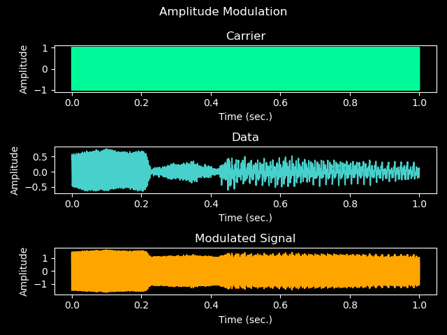
Figure 2.5 - AM Modulated Audio

Note: Yours may look different. I used a different audio file.

The carrier frequency (8000hz) is so high it appears as a solid block when plotted! This is normal, and you can see the amplitude changes of the data sinusoidal being represented as amplitude changes in the carrier signal in the modulated signal!

Now, looking at modulated through the time domain isn’t too useful when the data gets any bit more complex than a single tone. So, let’s export our generate signal to inspect it through other means! We’ll use IQ files!

Before continuing, please make sure you read over the IQ Files section

We will cover the rest in the Utilizing IQ Files in Python section.

Single Sideband Modulation

Single Sideband, or SSB is a modulation based off of AM. It was originally created as an improvement of AM, which as discussed before is pretty inefficient. SSB is a single sideband of AM with no carrier.

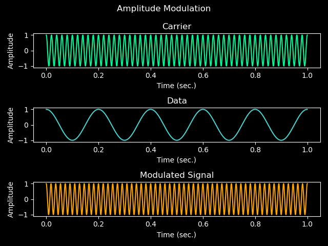
Figure 3.0 - SSB Graphs

As you can see, the modulated ssb signal is the carrier frequency offset by the data. Since AM was the sum and the difference of the frequencies, SSB, more specifically Upper Side Band, is purely the sum. There is also Lower Side Band, which is just the opposite.

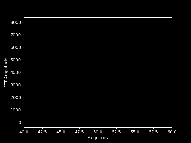
Figure 3.1 - SSB FFT

You can see the single tone in the frequency domain withh 100% power.

SSB comes at a disadvantage, where it is majorly more difficult to tune recieve because of the lacking carrier. The smallest of difference in LO frequency can make voice unintelligible. This is well documented in the Wikipedia SSB entry.

Despite this, SSB is currently the most popular mode in amateur radio due to its high power density and narrow bandwidth.

Math behind SSB

In principle, SSB is just the baseband signal with a imaginary component identical, but phase shifted 90 degrees

\[m(t) = s(t) * cos({2}\pi{ft}) - \hat{s}(t) * ({2}\pi{ft})\]

Here, \(s(t)\) is the baseband signal, \(f\) is the carrier frequency, and \(\hat{s}(t)\) is the Hilbert Transform of \(s(t)\). I don’t understand the Hilbert Transform, but all you need to know is that is shifts the phase of the input by 90 degrees.

We can simplify the above equation to use complex values, rather than handle both real and imaginary components individually. You’re gonna need to know this, for this part, and analytical signal is just a complex number with no negative frequencies; just a real signal and it’s Hilbert Transform.

We’ll call the analytical signal of \(s(t)\) \(s_a(t)\).

\[s_a(t) = s(t) + j * \hat{s}(t)\]

Where \(j\) is just the imaginary unit. \(s_a(t)\) now hold both the real and imaginary components of \(s(t)\). It’s complex! Now, according to Euler’s formula, quadrature carriers can also be represented analytically.

\[e^{ix} = cos(x) + isin(x)\]

Going off this, we can now represent out carrier as

\[e^{j{2}\pi{ft}}\]

Here, \(e\) is Eulers’ Number. I also found this representation of Euler’s formula pretty cool: Figure 3.2 - Rising circular

Now knowing all of this, we can convey

\[m(t) = s(t) * cos({2}\pi{ft}) - \hat{s}(t) * ({2}\pi{ft})\]

as

\[s_a(t) * e^{j{2}\pi{ft}}\]

You can also do Lower Side Band, but i’m not going to go into that today. Go checkout the SSB Wikipedia page for more.

SSB in Python

I’m hoping you read over the previous section about AM in python.

After importing numpy, we will start with our carrier and data signal. I’ll do both forms we went over in the math section.

import numpy as np

sampling_rate = 8000
duration = 1
t = np.arange(0, duration, 1/sampling_rate)
data = np.cos(2 * np.pi * 5 * t)

complex_data = np.hilbert(np.cos(2 * np.pi * 5 * t))
# OR
complex_data = np.cos(2 * np.pi * 5 * t) - 1j * np.sin(2 * np.pi * 5 * t)

# Carrier wave
carrier_freq = 50
carrier = np.exp(1j * 2 * np.pi * carrier_freq * t)1
# OR
carrier = np.cos(2 * np.pi * carrier_freq * t) + 1j* np.sin(2 * np.pi * carrier_freq * t)

Modulation is as simple as multiplying the data by the carrier.

modulated = complex_data * carrier

Let’s add the graphing stuff in too

fig, (ax1, ax2, ax3) = plt.subplots(3,1)
fig.suptitle("Amplitude Modulation")
fig.set_tight_layout(True)

ax1.plot(t, carrier, color="mediumspringgreen")
ax1.set_title("Carrier")
ax1.set_xlabel("Time (sec.)")
ax1.set_ylabel("Amplitude")

ax2.plot(t, data, color="mediumturquoise")
ax2.set_title("Data")
ax2.set_xlabel("Time (sec.)")
ax2.set_ylabel("Amplitude")

ax3.plot(t, output, color="orange")
ax3.set_title("Modulated Signal")
ax3.set_xlabel("Time (sec.)")
ax3.set_ylabel("Amplitude")

Let’s run it! We should get an output similar to Figure 3.0 I challenge you to adapt this to take an audio file input! Here’s what I got:

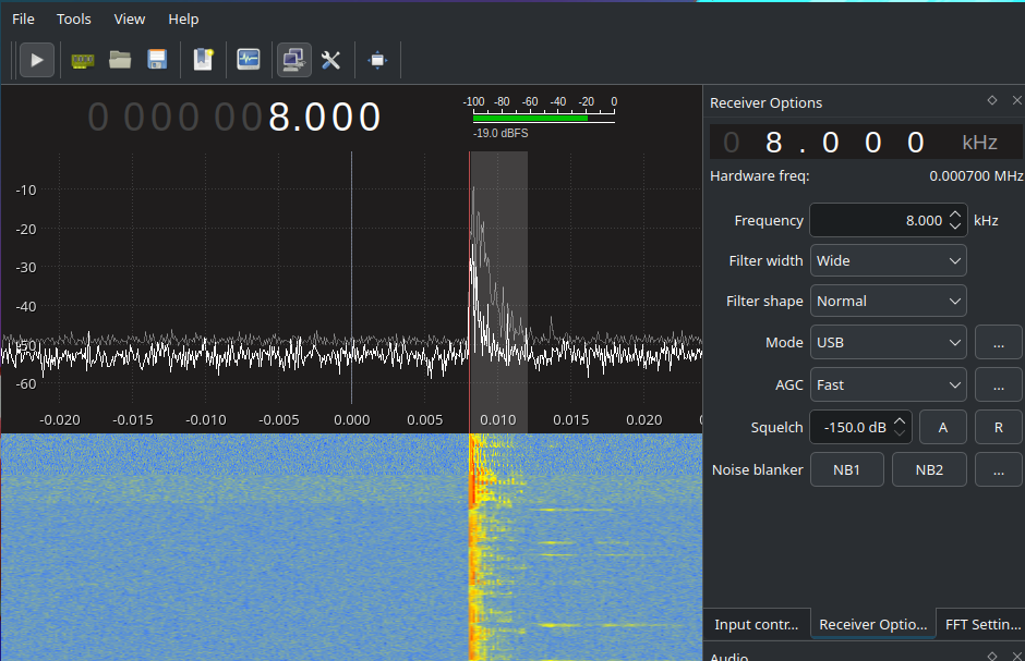
Figure 3.3 - SSB in GQRX

Note: I also added some noise to represent a real signal that a radio may receive!

Binary Phase Shift Keying BPSK is the simplest form of Phase Shift Keying, and transmits binary data between two distinct states in phase. It is widely used in digital communication.

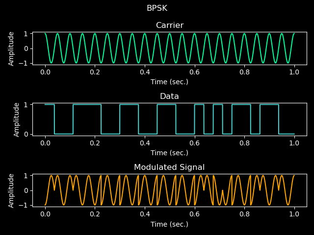
Figure 4.0 - BPSK Graphs

Notice the hard phase transitions? When looking in the frequency domain, this causes a lot of harmonic distortion.

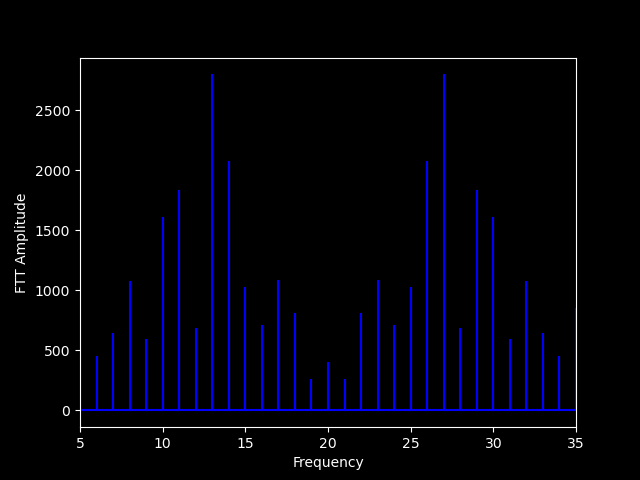
Figure 4.1 - BPSK FFT

In BPSK, phase is directly correlated to a 1 or a 0, For example a 0 could be 0 degrees and 1 can be 180 degrees. Another two popular choices are 45 degrees and 225 degrees. A receiver can then receive the bits and parse whatever format it is. We’ll be going over Varicose today, the format used in amateur radio.

Due to only two states, BPSK can only transmit 1 bit per symbol.

With digital modes, we now also introduce a new variable, the symbol rate. A symbol can be defined as a constant variable that lasts during that value’s duration. For example, If our symbol rate is 10, that means 10 different bits will be transmitted per second. With only two states in BPSK, the every symbol will convey 1 bit, and a single symbol will last \(1sec/10 = 0.1sec\). At 10baud (10 bits per second), 1 symbol will last 0.1 seconds.

When it comes to digital signals, we can also visualize their constellation! We can graph the I component as x, and the Q component as y.

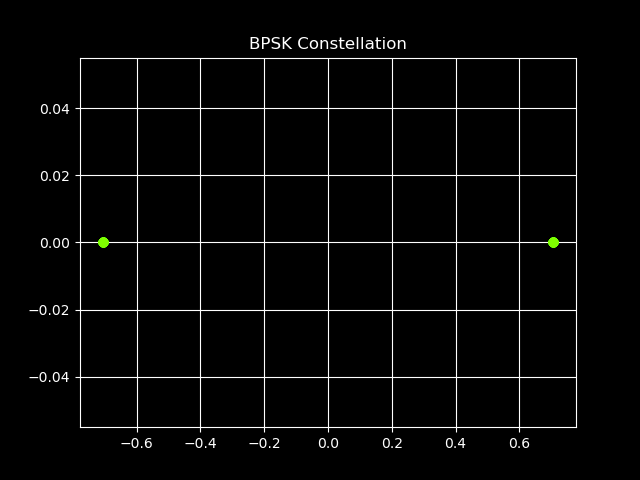
Figure 4.2 - BPSK Constellation

Here’s an example BPSK IQ constellation. We can see the two individual states of phase being 180 degrees out of phase. We can also look at another modulation, QAM and see how it has 4 states.

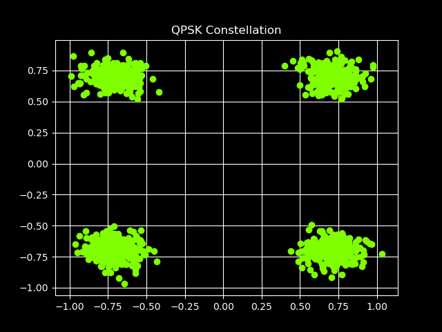
Figure 4.3 - QPK Constellation with noise

I also added some noise to this one to show what a more realistic signal may look like. This is QPSK, or Quadrature Phase Shift Keying. The BPSK constellation has two perfect dots because there is no noise present.

Math behind BPSK

Since BPSK is just 180 degrees phase shifts, BPSK can be represented as:

\[m(t) = cos({2}\pi{ft}+\phi{(t)})\]

Where \(\phi(t)\) is the phase as a function of time, either being \(\pi\) or \(0\).

The two different states can also be represented as:

\[ cos({2}\pi{ft}), n = 0\]

\[ cos({2}\pi{ft} + \pi), n = 1 \]

Creating BPSK signals in Python

Here, we’re gonna go a little above too! We’ll make a full-fledged BPSK implementation what uses Varicode, so we can actually communicate with other radio operators!

First, let’s get the basics in:

import numpy as np

sample_rate = 8000

And first, let’s make a function that takes in an array of “bits” and creates a BPSK waveform from it.

def gen_bpsk_waveform(bits, carrier_freq, symbol_rate = 31):
 symbol_len = int(sample_rate / symbol_rate)
 num_samples = len(bits) * symbol_len
 time = np.arange(num_samples) / sample_rate
 

 # Generate waveform
 data = np.array(bits).repeat(symbol_len)
 phases = np.pi * data
 output = np.cos(2 * np.pi * carrier_freq * time + phases)

 return output

And that’s really it.. Outputting and inspecting in software will be all as expected!

However, with modes like BPSK, it is customary to use Differential Coding. In its current state, if the receiver of the BPSK signal is exactly 180 degrees out of phase, or the polarity is reversed, the bit stream will be the opposite. 0101010 will look like 1010101, for example. Differential Coding makes the bits rely on the current and previous bit to make an unambiguous bit stream.

In Differential Coding, a high value marks a change in value, and a 0 mean it will stay the same. For example, representing 10010010 in differential coding will be 11011011. Let’s explain:

11011011 Bit 1 - Initial Value 1 Bit 2 - Change Value 1 Bit 3 - Keep Value 0 Bit 4 - Change Value 1 Bit 5 - Change Value 1 Bit 6 - Keep Value 0 Bit 7 - Change Value 1 Bit 8 - Change Value 1

Let’s implement this!

def differential_encode(bits):
 encoded = [bits[0]]
 for i in range(1, len(bits)):
 prev_bit = encoded[i - 1]
 current_bit = bits[i]

 if current_bit == 1:
 encoded.append(prev_bit)
 else:
 if prev_bit == 0:
 encoded.append(1)
 else:
 encoded.append(0)
 return encoded

Perfect! We can combine these together:

data = [1,0,1,0,0,0,1,0,1,0,1,1,0,1,1]
data = differential_encode(data)
modulated = gen_bpsk_waveform(data)

Let’s work on implementing Varicode now! Looking at the BPSK spec, we can see that every ASCII value has a corresponding Varicode value. We can represent this as a dict:

varicode_dict = {
 0: "1010101011", # 
 1: "1011011011", # 
 2: "1011101101", # 
 3: "1101110111", # 
 ...

}

I truncated it because it goes on for a while. Varicode is extremely well thought of in the way that different letters are actually of different lengths. More common letter have shorter transmission lengths, making the effective speed faster! For example, E is 1110111 while a is 1011. A space is also 1,

For this implementation, I’ll go through a string one character at a time, convert the char to varicose, then push the varicode to an array. Every message also begins with 20 bits of 0 and ends with 20 bits of 1

def string_to_varicode(text):
 bits = []
 # Preamble
 bits += [0] * 20

 # Data
 for char in text:
 varicode_str = varicode_dict[ord(char)]
 bits += list(varicode_str)
 bits += character_seperator

 # Postamble
 bits += [1] * 20

 return bits

Awesome! We can set our final implementation!

bits = string_to_varicode("BPSK31 Signal! We're transmitting text!")
bits = differential_encode(bits)
output = gen_bpsk_waveform(bits, 875)

Awesome! This is technically a full fledged BPSK application! However since the waveform is unfiltered, there will be a lot of harmonic distortion. this leaves to a bad experience for other operators.

I would go into filtering, but I really don’t understand it myself.

Utilizing IQ files in Python

For this section, I’ll be assuming all of the variable from the previous section exist.

I will not go over using SigMF in this section, primarily because I haven’t used it yet, by the PySDR book has a great section about this.

Binary Files

The easiest way to make an IQ file in python is to just export the data list as a complex64, which stores both I and Q components as a float32 in a binary file.

This is extremely simple using numpy, we just convert the data to complex64 and save it to a file.

output = modulated.astype(np.complex64) 
output.tofile("data.iq")

We now have our signal in an IQ file named data.iq!

You can also import this back into Python as such:

data = np.fromfile('data.iq', np.complex64)
print(data)

However, as said before, binary files contain no metadata. You may run across IQ files stored in Int16, which is also common. In this case, you can easily convert them as such:

# The python way
data = np.fromfile('iq_samples_as_int16.iq', np.int16).astype(np.float32).view(np.complex64)

# The traditional way
data = np.fromfile('iq_samples_as_int16.iq', np.int16) #IQ in int16
data = data / 2**15 # Normalize data = data[::2] + 1j*data[1::2] # convert to IQIQIQ...

Wave Files

IQ data in wave containers are also a common choice, and are almost exclusively stored in Int16. So, in order to store our samples in a wave file, we must first separate the I and Q components, convert them to Int16, and then store it into a two channel wav file.

# Write to WAV container
# Create I and Q signals
I_signal = (np.real(output) * 32768).astype(np.int16)
Q_signal = (np.imag(output) * 32768).astype(np.int16)

# Combine I and Q signals as stereo data
stereo_data = np.column_stack((I_signal, Q_signal))

# Save stereo wav file
wavfile.write('IQ.wav', int(sampling_rate), stereo_data)

You now have an IQ file at IQ.wav!

Visualizing Signals from IQ files

Inspectrum

A common way to visualize and analyze radio signals from IQ files is using software like Inspectrum. Go to the repository and install it for your distro!

I use arch, so installing looks as such for me:

$ sudo pacman -S inspectrum

With inspectrum installed, we can open our IQ file with it. Inspectrum supports all of these formats:

inspectrum supports the following file types:

• *.sigmf-meta, *.sigmf-data - SigMF recordings
• *.cf32, *.fc32, *.cfile - Complex 32-bit floating-point samples (GNU Radio, osmocom_fft)
• *.cf64, *.fc64 - Complex 64-bit floating-point samples
• *.cs32, *.sc32, *.c32 - Complex 32-bit signed integer samples (SDRAngel)
• *.cs16, *.sc16, *.c16 - Complex 16-bit signed integer samples (BladeRF)
• *.cs8, *.sc8, *.c8 - Complex 8-bit signed integer samples (HackRF)
• *.cu8, *.uc8 - Complex 8-bit unsigned integer samples (RTL-SDR)
• *.f32 - Real 32-bit floating-point samples
• *.f64 - Real 64-bit floating-point samples (MATLAB)
• *.s16 - Real 16-bit signed integer samples
• *.s8 - Real 8-bit signed integer samples
• *.u8 - Real 8-bit unsigned integer samples

If an unknown file extension is loaded, inspectrum will default to *.cf32.

Note: 64-bit samples will be truncated to 32-bit before processing, as inspectrum only supports 32-bit internally.

Sourced from the README.md

Let’s open inspectrum! inspectrum data.iq

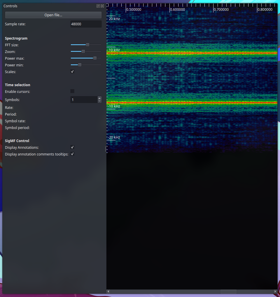
Awesome! After adjusting the sample rate, FTT, Zoom, and power, we can clearly see our AM signal at 8kHz, along with the two sidebands! Our signal is real! Next, let’s use SDR software to have some more control and fun with our signal.

GQRX

I won’t go too in dept in this section. If you wish to learn more, please look at the GQRX documentation.

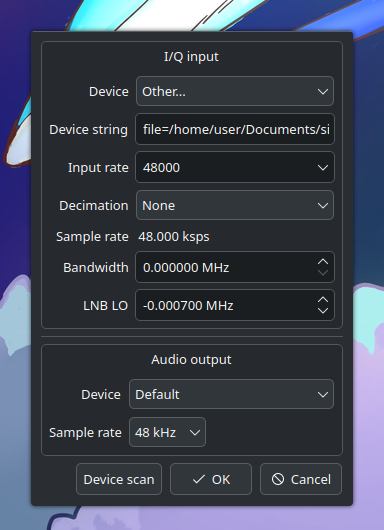
After installing GQRX and opening it, a menu like this will appear: Figure 3.0 - GQRX Config Dialog

Here we will set the Input Rate (the sampling rate) at 48000hz. If this value is incorrect, the signal will be all incorrect. In the Device string section, just change the file parameter to wherever your binary IQ file is. GQRX takes in a 32bit binary file as specified in the binary files section. Click OK and then you’ll be brought to the main GQRX window.

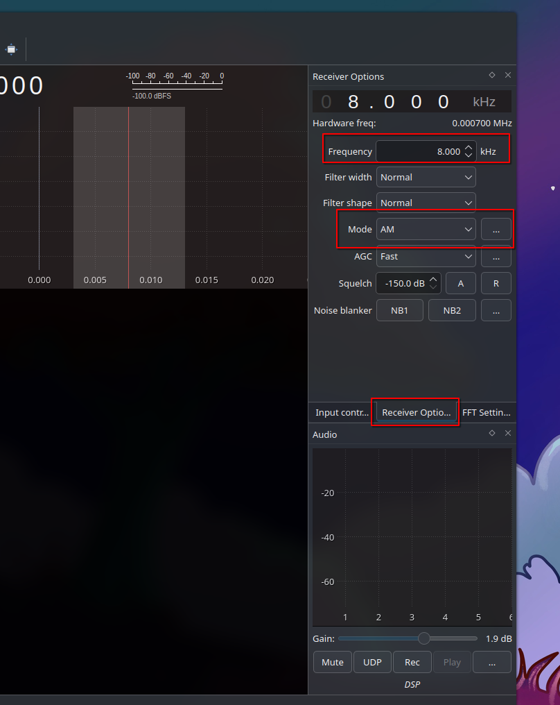
Figure 3.1 - GQRX Reviever Options

Be sure to configure the Reciever options as shown in the photo!
Click the start button on the top left of the window, and you will now see and hear your modulated signal.

Note: Notice how there’re two signals, one at 8khz and -8khz?

You many notice (thanks to he note above) that there are two identical signals, one at 8kHz and one at -8kHz. What gives? This is because our Q channel is actually empty All we have is the I channel, which is not enough information to properly convey a complex signal. If our Q signal was identical to the I, but 90 degrees out of phase will result in a proper result. This can be done using a Hilbert Transform

TL;DR

This post was intended to be an introduction to DSP and SDR. I will post at minimum monthly posts now describing more SDR and DSP techniques, and progress on my transceiver! Since this post covered a lot of the software side of this stuff, I hope to next make a post going over the hardware side of this. Soon we van make a post about interfacing with a RTL-SDR and make some demodulators.

I didn’t really expect to write this much.. But I hope it can be a good resource :)

All code used to create this, including graphs and stuff is avaliable at this repo.

Thank you for reading :)

dragongoose loves you!